
If you’re looking into help desk jobs but aren’t sure your resume is worth anything because you have no prior professional IT experience, think again.

Healthcare workers play an important role in society. But we completely understand that it is easy to get burned out or overwhelmed in this demanding
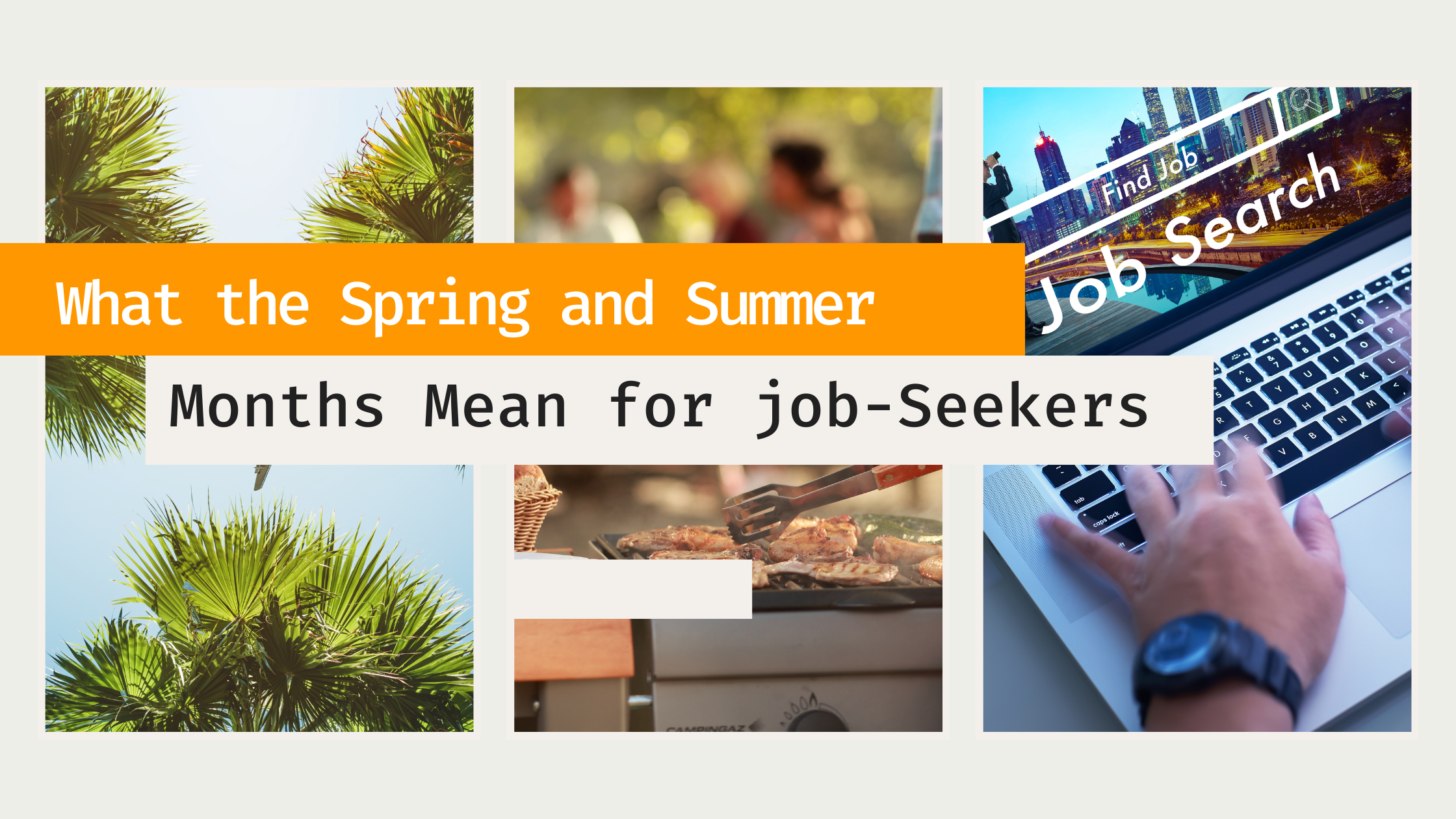
The warmer months aren’t just for vacations and throwing food on the grill. For job seekers, especially those in tech, spring and summer can be
If you’re looking into help desk jobs but aren’t sure your resume is worth anything because you have no prior professional IT experience, think again.
Healthcare workers play an important role in society. But we completely understand that it is easy to get burned out or overwhelmed in this demanding

Tech School vs College It’s a common misconception that the only way to enter the workforce is to have a college degree. Most high school

Are you overwhelmed by the thought of creating videos for your business? Questions like what to talk about, who should be in it, where to
Are you ready to captivate your audience with engaging video content? You don’t need complex and lengthy productions to make an impact. In fact, it’s

Traditional advertising methods no longer possess the same influence they once did. If you’re looking to captivate your target audience and supercharge your sales, it’s
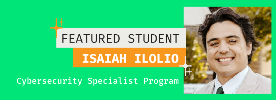
Centriq recognizes 1-2 outstanding students as our Featured Student of the Month. Isaiah Ilolio is one of our Featured Student of June 2025. Get to

Centriq recognizes 1-2 outstanding students as our Featured Student of the Month. Trey Dyer was awarded our Featured Student of June 2025. Meet Trey, one
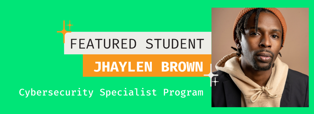
Centriq recognizes 1-2 outstanding students as our Featured Student of the Month. Jhaylen Brown was awarded our Featured Student of May 2025. Meet Jhaylen Brown, a

Centriq’s New AI Hub: How SMBs Are Winning with a Secure, Scalable AI Strategy “I know I should be doing something with AI… I’m just

AI: Your Business’s New Best Friend (Not Your Replacement) AI technology has become a powerful partner for small and medium-sized businesses. It’s not about replacing

Did you know that almost half (44%) of business leaders aren’t sure if their employees use AI tools at work, or how often they’re using
Centriq recognizes 1-2 outstanding students as our Featured Student of the Month. Isaiah Ilolio is one of our Featured Student of June 2025. Get to
Centriq’s New AI Hub: How SMBs Are Winning with a Secure, Scalable AI Strategy “I know I should be doing something with AI… I’m just
Centriq recognizes 1-2 outstanding students as our Featured Student of the Month. Trey Dyer was awarded our Featured Student of June 2025. Meet Trey, one